
Continued from Part I
Part I of this article appeared last week. In it I introduced the topic of statistical vs biophysical approaches to biological applications. I discussed the huge power of statistical approaches in image analysis and providing decision support services to doctors. I then discussed the 5 major limitations of data-driven approaches when they are applied to biological problems.
I will now continue by looking at biophysical approaches, their pros and cons, and finishing up with a brief introduction to hybrids which attempt to combine these two methods.
Biophysical approaches to biology
This is probably the space I have spent the most time working in throughout my career. I am not a physicist. I don’t excel at writing down equations for the underlying ionic currents and then connecting them to equations. I find that aspect a bit boring. But I have worked with the equations that others have written. I have scaled them up and used them as components in stochastic processes. And I have written my own phenomenological (not technically biophysical) equations to describe and study biophysical processes.
I will now give three examples, that I have personally worked on, incorporating these approaches at different levels of biological description and how these techniques have been particularly useful in applications.
Example #1
In sports science the lactate threshold of an athlete is considered to be a good proxy for their fitness. A simple thumb prick blood test can be analysed and the concentration of lactic acid in the blood is plotted against workload on a stepped workload protocol. For low workloads the blood lactate concentration is approximately constant. Then, above a certain point it appears to increase exponentially in response to increases in workload. Beyond this turning point the ability of the athlete to sustain increased workloads is greatly impaired.
The phenomenological understanding is that below the turning point the body is capable of buffering or clearing the increased levels of lactic acid which are being produced by the energy burning process. But once you go beyond this point the clearance processes have more or less maxed out.
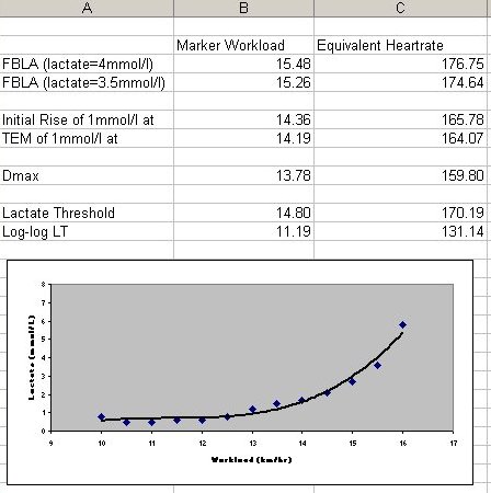
The lactate threshold of the athlete is the turning point mentioned above. But before we came to the field there was no true mathematical definition of this turning point. Coaches typically drew the experimental results, manually, on graph paper and visually identified the point of interest. There was no consistency, either between coaches or indeed across time from the same coach.
What we did was mathematise this process. The details are not strictly relevant here, what is important is that given the biological understanding of what was going on, and also of why it was relevant, we were able to write a formal mathematical description of the data and use this to automate future analysis. The software is freely available and is used in sports science labs throughout the world.
Example #2
Since the early days of neuroscience physicists have worked closely with experimental neuroscientists to develop biophysical equations for how the neuron works. It is standard practice for most beginning computational neuroscience students, at some stage, to attempt to fit some experimental data to a neuronal spiking model.
The actual biophysical models range from the highly detailed, often dividing up a neuron into small segments, to the highly abstract (leaky-integrate-and-fire, Linear-nonlinear-Poisson). Fitting them requires first choosing the appropriate level of abstraction. The practitioner is then left with an equation with a fixed number of parameters and a data set to which they wish to fit it.
In practice, some parameter values are known or can be fixed by other experiments. This leaves a smaller number of parameters which must be inferred from the data set. This is a standard optimisation problem (likely a nonlinear optimisation problem) and can be tackled by coupling the appropriate optimisation algorithms with the biophysical equation and using distance from the recorded data set as a success metric.
At this point scientists have gotten pretty good at reproducing the experimental data using fitted equations. These equations are used i) to validate our understanding of the underlying physiology, and ii) to predict outcomes to inputs which we have not observed, or not been able to observe, in experiments.
Example #3
The brain contains on the order of 10^9 neurons, so occasionally it is useful to look at what more than one neuron does at a time. It is possible to couple 1000s of equations of the type fitted in example #2. Each of these equations represents the activity of a single neuron. But we don’t fully know how the neurons are wired together yet, nor all of the neuronal types (which presumably will have different parameter values). So if we were to start trying things out using numerical simulations we might be here until eternity before we have a working system.
Luckily, there are two shortcuts available. Firstly, we can make some good approximations and guesses and formalise these in the initial setup. More importantly, we can use advanced methods from stochastic processes (eg. Focker-Planck equations) to predict the outcome of coupling the biophysical equations without needing to simulate a system of 1000s of coupled differential equations.
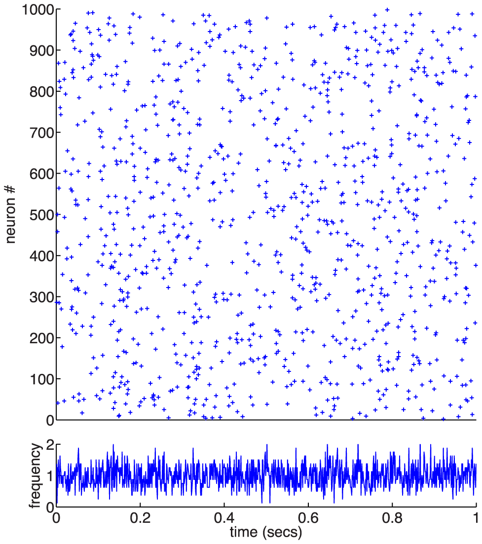
Using these advanced approaches we can setup the parameters in our equations in order to ensure any population behaviour we desire. In the example figure we see neurons firing randomly (Poisson process) at 1/sec with a known (and predicted) variance.
We can use these equations in two directions: i) downwards, in order to setup a network with desired behaviour, this is very important for testing theories for memory encoding, ii) upwards, we can save ourselves a lot of simulation work and just replace the whole system with a single equation!
Why don’t we see more of these pure modelling approaches?
I began by saying that I have spent considerably more of my time in the past 15+ years using biophysical (or as I sometimes call them ‘pure modelling’) approaches. So are these really the best approaches?
Betteridge’s law of headlines implies that the answer here is No. Let’s look here at what is wrong with biophysical modelling approaches.
We can summarise the problems pretty quickly:
- The techniques are technically quite difficult and the expertise not widely available.
- Fitting the equations typically tends to apply only to the experiments from which the original fit was acquired and is not necessarily generalisable.
- Coupling equations which were fitted using data from different experiments, in different labs, at different times, rarely works.
The technical difficulty should not be underestimated here. In the examples I presented above, all of which I have personally worked on, it is almost unheard of to have a single expert who can work on all three of those projects. That means that normally, either i) you hire the expert first and allow them to focus the project on the techniques in which they are expert (the most common approach in academia), or ii) you find a CTO (because this is an industrial approach) who has enough knowledge of the separate techniques in order to frame the project and you have enough money left over for them to hire the expertise that is needed at each stage in the project.
The inability to generalise from biophysical equations is disappointing given my complaints about a similar problem in data-driven models in part I of this article. In this case, however, this is probably an unfair comparison. With blackbox data-driven models we have no idea where it might go wrong and no way to recognise it when it does. With biophysical models we have the full mechanics of the model at our fingertips. An expert can and will see the problem pretty quickly. But you need to be an expert in order to do this!
Finally, the fitting of equations is very dependent on conditions under which the data was acquired. Given, again, the issue of noise in biology it is entirely possible that: on day 1 the data was sampled from the left-skew of an underlying distribution; on day 2 the data for a separate fit from the right-skew. If you could have collected both sets of data from their true underlying distributions you would have had no problem. But if these are coupled processes, in the biology, you may not be sampling from the same sample noise regime when gathering the data. In this case, it is not surprising that you get weird results when you couple the fitted equations.
Of course, the real cost of using these techniques is that they require huge amounts of expert knowledge and are time consuming to implement.
Hybrid approaches
Data-driven approaches are great because they are quickly turning into turnkey solutions. However they have issues with applicability in biology.
Biophysical, or pure modelling, approaches have massive overheads in terms of time and expertise but can help to overcome issues of sample size and noise.
Despite the long history of separation between these different approaches there is now an emerging sector which attempts to combine them. For a long time this was considered a risky approach. Until recently, data-driven approaches were still extremely difficult to implement. This required separate sets of experts working on both sides of the problem.
With the advent of relatively simple libraries which automate the implementation of data-driven approaches (eg. PyTorch) it has become considerably easier for non-experts to roll-out such solutions. Issues of interpretation still exist, but for now they are largely swept under the hype-driven carpet.
The goal of hybridising these two approaches is to benefit from a best-of-both-worlds situation. Data-driven approaches can be rolled-out easier, can be implemented by engineers, and they quickly capture high-dimensional correlations which humans would be likely to miss. But, since the sample size in biology is low, some bespoke biophysical models can be used to bootstrap the approach.
The example with which I have most familiarity is that of the Prediction 2020 project which is currently being spun-out of the Charité hospital via its BIH incubator. (Prediction 2020 is not my project, I have never worked on it, my familiarity ends at a number of public presentations I have attended and I do happen to know some of the team personally.) The goal of the project, as far as I understand, is to take MRI images of stroke patients and to predict how much further damage they are likely to have in two cases, i) if they receive no further treatment, and ii) if they receive a drug which has a 15% likelihood of causing severe, life-threatening side-effects. The project output is a product which can be used in a clinical decision support setting; allowing doctors to better treat stroke patients.
Now, with pure machine learning approaches it is pretty hard to build a decent classifier from only ~300 training images. This is especially the case when the stroke will have occurred in different locations for different patients. You are almost in the realm of n=1 for each of the cases of interest. As I argued, quite expansively in part I, the fact that an MRI is extremely rich in data is more correctly treated as high-dimensionality in this case and cannot be transformed into extra training points.
The Prediction 2020 project, quite intelligently, augments the inputs to their machine learning classifier by simulating blood perfusion locally, throughout the brain, based on a vascularisation scan. By building-in biophysical knowledge into the simulations they are better able to leverage latent aspects of the blood flow data from the MRI scans; effectively lowering the signal-to-noise ratio.
My own company, Simmunology, is flipping this approach on its head. Whereas Prediction 2020 are feeding the simulation results into the machine learning methods, we are using Deep Neural Networks at the lower level, using this to drive higher-level structural elements which we use to describe the Human Immune System.
Conclusion
A practitioner should always know their tools. We are currently seeing an unprecedented gold-rush in the application of Deep Neural Networks to industrial problems. Investors see the potential for revolution, but don’t know enough about the techniques to sort good investments from bad.
Data-driven techniques come with some quite specific characteristics (see part I) which limit their applicability to biology and healthcare applications. This does not mean that they should not be used. But it does mean that those limitations should be accounted for before deciding to throw a lot of time and money at a problem.
Biophysical modelling approaches, by their necessity, will always require some degree of heavy lifting. This is unattractive during a gold-rush. However, the low-hanging fruit of biomedical development have already largely been picked. Anyone wishing to make further advances in healthcare and drug development will have to accept that this is not a field where results just appear magically overnight. That said, these techniques are often overly bespoke and lack the possibility of being repurposed quickly into other products.
Thankfully, we don’t have to resign ourselves to a world in which we must choose between shallow solutions which limit our future progress and deep solutions which take decades to implement. There is a sweet spot in-between. The formerly separated (academic) fields can come together, and appear to be doing so in the industrial context. A hybridisation does require even greater ability, at least to communicate, at the direction-level. But making it work, and work well, at the implementation-level is considerably easier. This will allow us to make swift improvements in healthcare applications in the coming 3 to 5 years.
One Reply to “AI in Healthcare II”